¶ Software Manual
Version 1.0 Last Revised 25.01.2021
All contents in this manual are copyrighted by JAVAD GNSS. All rights reserved. The information contained herein may not be used, accessed, copied, stored, displayed, sold, modified, published, or distributed, or otherwise reproduced without express written consent from JAVAD GNSS.

¶ Introduction
Automonitoring software implements the innovative method of estimating point displacements by processing measurement data streams from standalone GNSS receivers.
The main estimated parameters are the changes of receiver position over a standard (1 sec) time interval, i. e., in fact, the components of receiver velocity. Accumulating one-second position changes, or which is the same as integrating the velocities allows calculating receiver displacement over time.
The Automonitoring performs an independent estimation of the displacements for each monitored point. As research shows, to achieve millimeter level accuracy of the automonitoring, it is sufficient to use broadcast ephemeris received by the standalone receiver, and its double-frequency phase measurements.
So this method of monitoring displacements is fully autonomous because it does not depend on data from other receivers, precise ephemeris, or any additional external information. The only one-second data stream of autonomous double-frequency monitored receiver is needed.
Processing of GNSS data streams from each monitored point is carried out by a separate processor that accounts for specific observation conditions (that is, multipath, sky closure, etc.). The distance from the processing center and the monitored receiver can be arbitrary, provided that there is a reliable Internet connection.
¶ The graphical user interface
¶ Settings
The Settings screen is used to enter settings that are common to all monitored points.
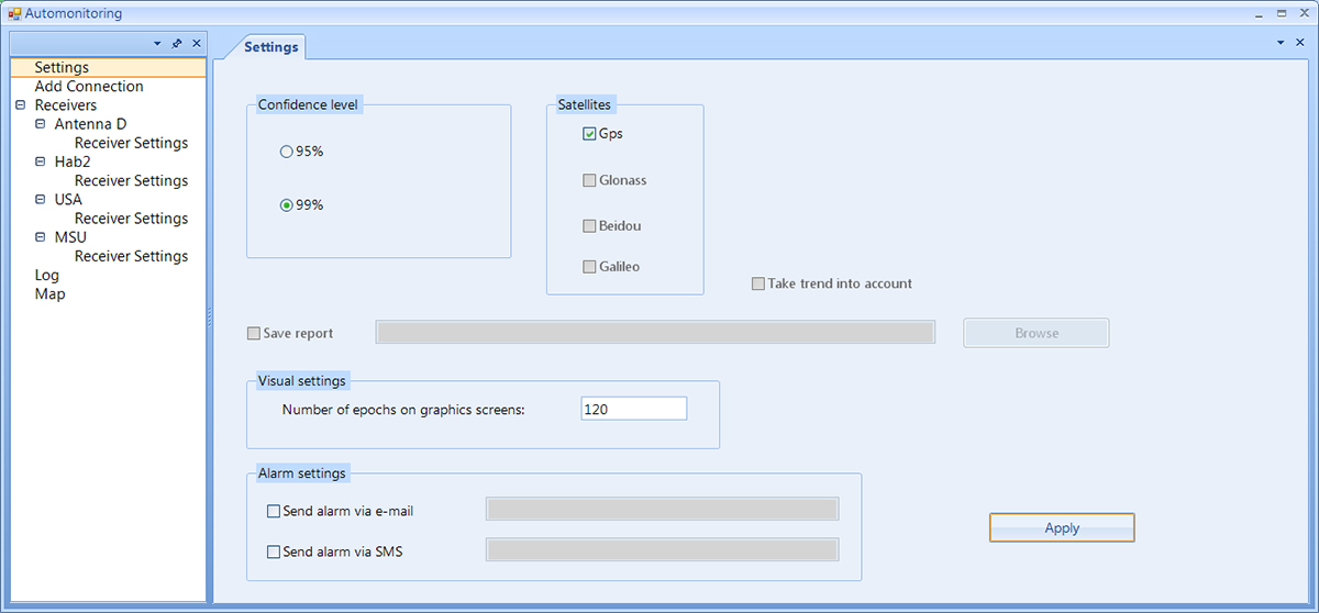
Figure 1. Settings
- Confidence level – selection of a confidence interval for detecting and filtering outliers using statistical methods.
- Satellites – selection of the GNSS system.
- Take trend into account – taking into account the erroneous linear trend of the accumulated position displacements.
- Save report – address for saving the monitoring report.
- Visual settings – graphical settings (how many measurement epochs to show on the screen at the same time).
- Alarm settings – addresses for sending alarm messages by e-mail or SMS.
¶ Add Connection
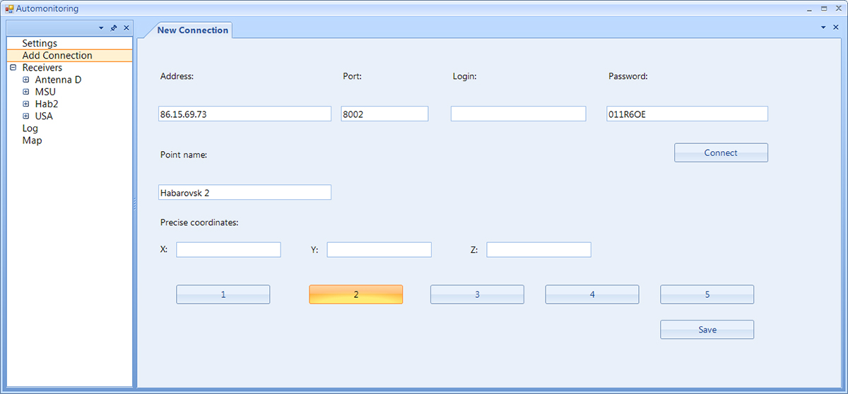
Figure 2. Add Connection
- Address, Port, Login, Password – parameters for connecting to the receiver to access the GNSS measurement stream.
- Point name – the name of the monitored point.
- X,Y,Z – fields for entering the point’s precise coordinates at the initial epoch of monitoring. If not entered, the program uses the receiver’s standalone coordinates.
To start to work with receiver click Connect.
¶ Monitored points and used receivers
The Receivers screen lists the monitored points as well as the addresses and models of their receivers.
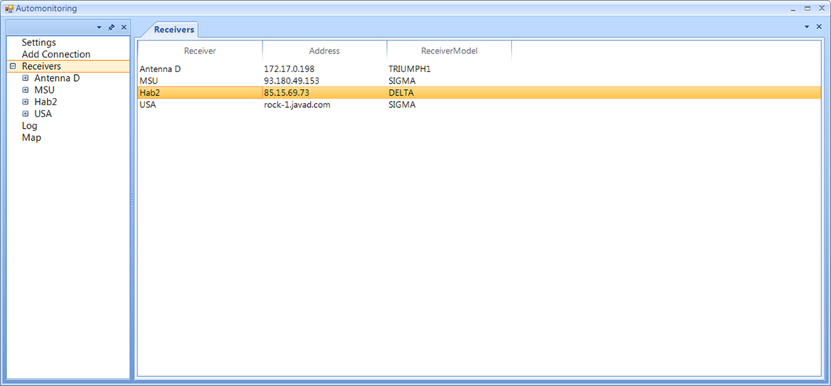
Figure 3. Receivers
¶ Receiver Information
The Receiver information screen contains detailed information about monitoring points.
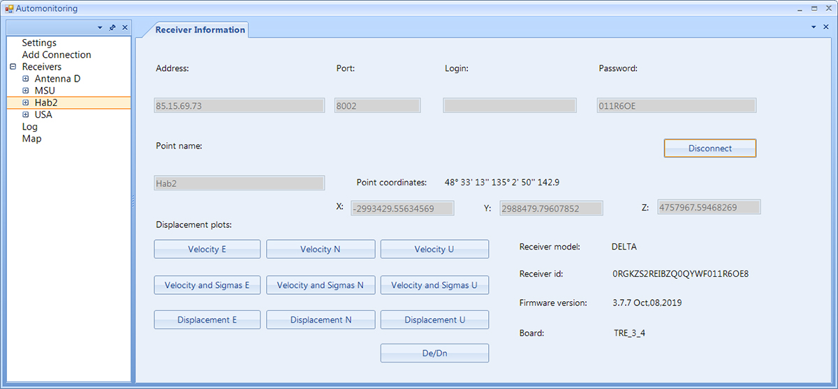
Figure 4. Receiver Information
The top of the Receiver Information screen contains the information entered earlier in the Add Connection screen:
- Address, Port, Login, Password – parameters for connecting to the receiver to access the real-time GNSS measurement stream.
- Point name – the name of the monitored point.
- Point coordinates – geodetic and rectangular coordinates of the monitored point.
- At the bottom of the screen оn the right, the receiver parameters are shown (receiver model, receiver id, firmware version, board).
- At the bottom of the screen on the left, there are buttons for displaying displacements of monitoring plots. Two types of plots are shown - velocities and accumulated displacements.
- Velocity E, Velocity N, Velocity U - plots of measured velocities of displacements in the east, north and vertical directions:
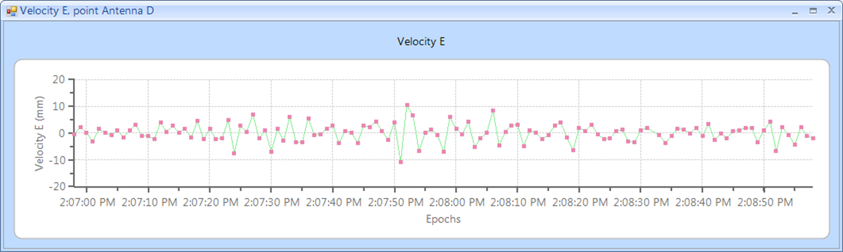
Figure 5. Plots of measured velocities
- Velocity and Sigmas E, Velocity and Sigmas N, Velocity and Sigmas U – plots of velocities, as well as their measurement errors, with the addition of two horizontal lines showing the geometric thresholds for allowable displacements that are set on the Receiver settings screen:
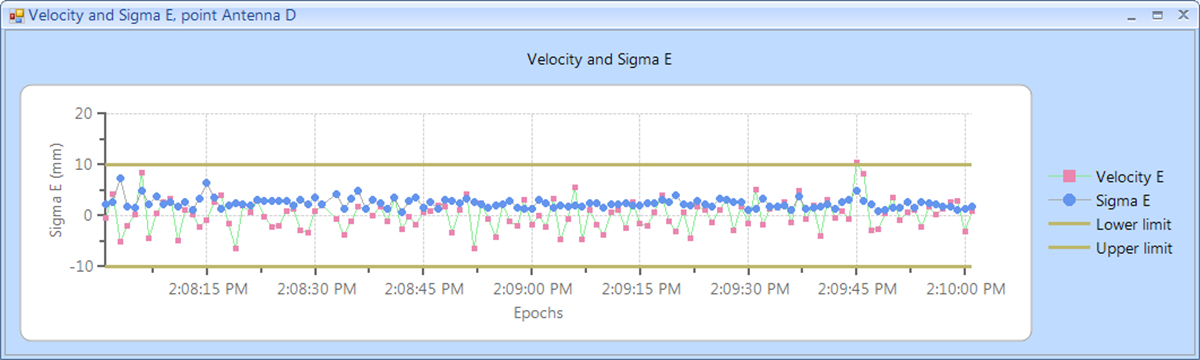
Figure 6. Plots of measured velocities and their accuracy estimates
- Displacement E, Displacement N, Displacement U - plots of accumulated displacements of the point in the east, north and height directions:
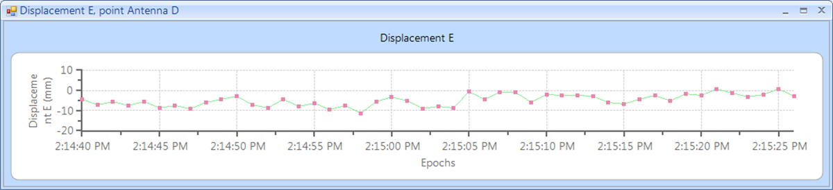
Figure 7. Plots of accumulated displacements
- An additional DE/DN plot shows the accumulated displacements of a point in the horizontal plane:
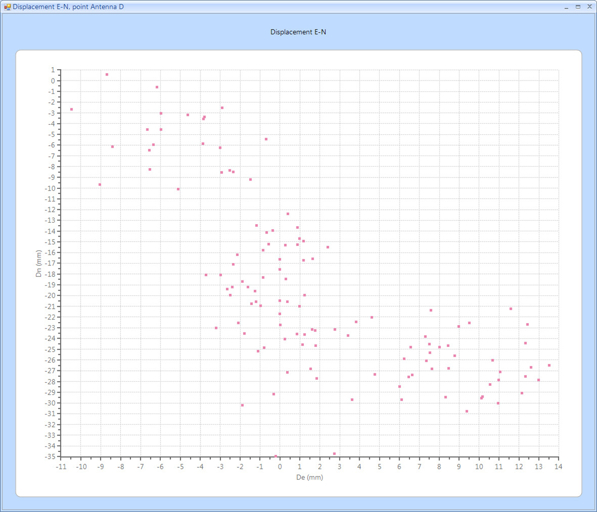
Figure 8. Plot of accumulated displacements (in horizontal plane)
The displacements are accumulated starting from the moment of the “red” level, when any of the velocity components begins to exceed the acceptable threshold, that is, when a sequence of statistically significant abnormal velocities occurs. The program begins to integrate velocities and draw plots of the displacements of a given point in all three directions - east, north, and height.
When all three velocity components return to acceptable limits, the displacement accumulation plots are no longer displayed.
¶ Receiver Settings
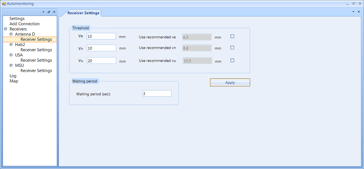
Figure 9. Receiver Settings
On the Receiver Settings screen, you can set the permissible thresholds of displacements (Thresholds), as well as the Waiting period - the allowable time interval between the moment of detecting the displacement and the moment of generating an alarm message.
Note: These thresholds are set independently for each receiver, since the observation conditions at the monitoring points may differ.
To help the user who may not know precisely the real observation conditions (the multipath, etc.), and therefore cannot set realistic values for displacement thresholds, the program estimates itself the accuracy of measured velocities at each monitored point.
On the right side of the screen, the fields Use Recommended ve, Use Recommended vn, Use Recommended vu are shown. They show the values of the permissible displacement thresholds estimated by the software during the processing of GNSS observations made at this point for several hours. At the end of this estimation interval, the recommended Thresholds values appear in the corresponding fields. If they are accepted, you need to tick the check boxes and click Apply.
¶ Monitoring Log
The monitoring log records significant monitoring events for all monitored points, such as:
- missed measurements, and their resumption;
- the probable beginning of the point displacement process;
- the confirmed beginning of the point displacement process;
- the possible completion of the point displacement process;
- confirmed completion of the point displacement process;
- changing by the user the allowable thresholds in the Settings;
- text of alarm messages (Alarms) sent by SMS or e-mail.
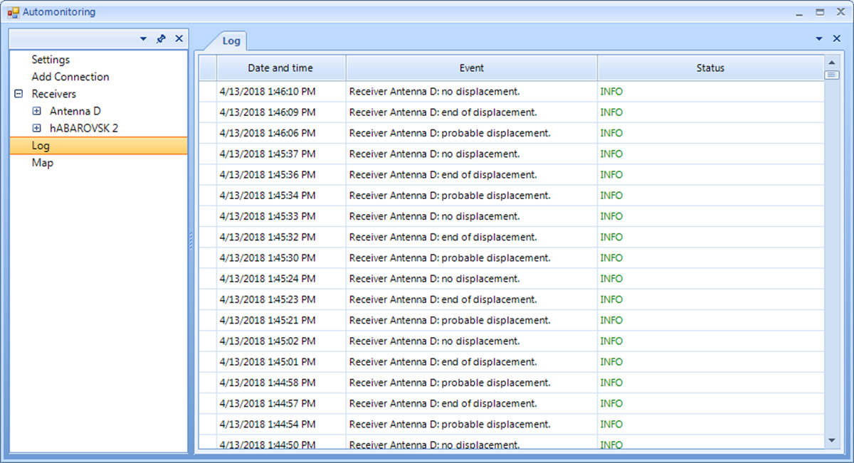
Figure 10. Monitoring log
¶ Map
In addition to tracking monitoring plots, the program presents the active map that shows all the monitoring points. With the use of traffic light symbols color indication, their stability is shown in real-time.
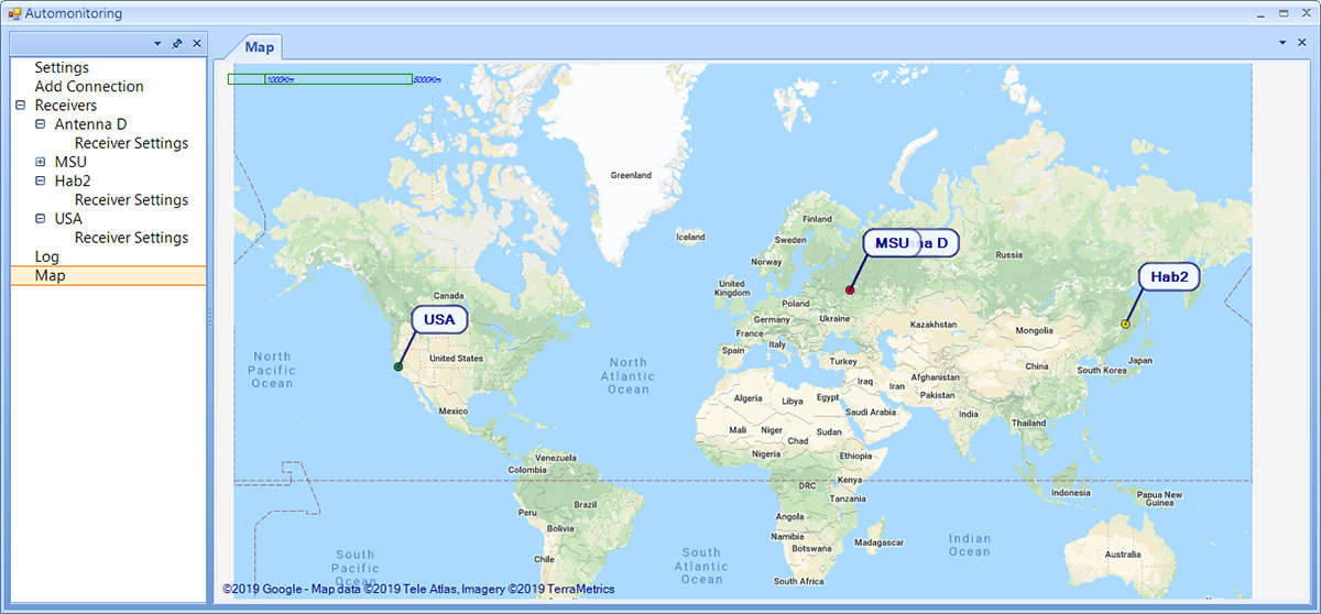
Figure 11. Active map of monitoring
Each point can be shown in three states:
- The point is stable (i.e., no displacements were detected). In this case, the monitoring point is shown on the map in green.
- The probable point displacement is detected. In this case, the yellow color lights.
- A confirmed displacement has occurred. The point is shown in red.
Waiting time (permissible duration of yellow light before lighting red) - that is, the probable displacement period - is set in the Receiver Settings by the value of the Waiting period interval. The yellow light will remain on for the same amount of time after the end of the confirmed displacement period (i.e. after the end of the red light). Then, when the point returns to a stable state, it is shown in green.
900 Rock Avenue, San Jose, CA 95131, USA
Phone: +1(408)770-1770 Fax : +1(408)770-1799
www.javad.com
All rights reserved © JAVAD GNSS, Inc., 2020